
Advection schemes#
TRACMASS-JAX has the two trajectory schemes of Fortran TRACMASS. You choose
one with scheme= in steady_state and time_dependent:
|
Fortran module |
JAX factory |
|---|---|---|
|
|
|
|
|
|
The factories live in tracmass.advection_scheme. In the time-stepping
scheme the fluxes are frozen during a sub-step and interpolated in time
between sub-steps. In the time-analytical scheme they vary linearly in time
inside the step.
Both factories close over the GridFields, compile with jax.jit, and
return
step_all(fluxes, state, intrpg, dsmin) -> ParticleState
which advances every active particle by one sub-cycle. The per-particle
work is done by _subcycle_one_particle (or its analytical twin) mapped
over the particles with jax.vmap. The patched and streaming integrators
use the same equations through piecewise_local and piecewise_stencil
(see Integrators).
Each sub-cycle works like update_traj, cross_time and calc_pos in the
Fortran code:
Interpolate the face fluxes in time.
Compute, for each of the six faces, the time the particle needs to reach it (
cross_time).Take the smallest of those times and the step cap
dsmin.Move the particle for that time (
calc_pos) and, if it reached a face, move it into the neighbouring cell (update_traj).Stop it if it ended up on land, outside the domain, or in a cell with no volume.
Volume-normalised time#
The schemes work with the time-like variable
so that a volume flux \(U\) (m³ s⁻¹) in index space moves a particle by
\(\mathrm{d}r/\mathrm{d}s = U\) cells. In the code \(\Delta V\) is
dxyz = dxdy * dzt * zstot, interpolated in time with each particle’s own
weight. A step ds corresponds to a physical time dt = ds * dxyz. The
step cap dsmin, the time left until the particle’s next sub-step boundary,
is converted to dsmin / dxyz before the crossing times are compared.
Time interpolation#
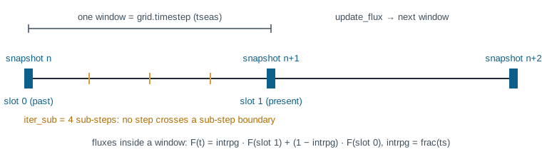
A window lies between two GCM snapshots \(t_0\) (slot 0) and \(t_1\) (slot 1). The fluxes on each face are interpolated linearly in time:
The weight intrpg is the fractional part of the normalised time ts
(time in units of the GCM timestep). Like the Fortran code, the
time-stepping scheme uses one weight for all particles in a sub-cycle:
the mean ts of the active particles. A per-particle weight lets the
interpolated flux at a wall change sign between consecutive sub-cycles,
which makes particles bounce back and forth across the wall. The cell
volume dxyz uses each particle’s own weight, because it only affects the
step cap.
Time-stepping scheme ("tstep")#
Within a sub-step the fluxes are frozen at their time-interpolated values.
Consider the zonal direction in cell ia, which covers
\(x_W = i_a - 1 \le x \le x_E = i_a\), with flux \(U_W\) on the west face
(um) and \(U_E\) on the east face (uu). TRACMASS assumes the flux varies
linearly across the cell:
With \(\mathrm{d}x/\mathrm{d}s = U(x)\), this gives an exponential solution in \(s\).
Crossing time (_cross_time_1d, Fortran cross_time)#
For a particle at \(x_0\), the time to reach the east face, dse, exists
when \(U_E > 0\):
and it is UNDEF (\(10^{20}\)) otherwise. The time to reach the west
face, dsw, exists when \(U_W < 0\):
Non-positive results are set to UNDEF. The same function gives dsn and
dss from vflux, and dsu and dsd from wflux.
Step length#
The step is the smallest of the six crossing times and the cap:
The face that sets \(\Delta s\) decides where the particle goes, as in the
Fortran update_traj:
Limiting time |
New cell |
Boxface |
|---|---|---|
|
|
1 east |
|
|
2 west |
|
|
3 north |
|
|
4 south |
|
|
5 |
|
|
6 |
|
unchanged |
0, still inside the box |
If every crossing time is UNDEF (a convergence zone) the particle stays
in its box for the whole step. When two faces are reached at the same time
(a corner), the particle moves diagonally only if the diagonal cell is
ocean.
New position (_calc_pos_1d, Fortran calc_pos)#
After a step \(\Delta s\) the new position is
and the same for \(y\) and \(z\). On the face that set the step, the position is set exactly to the wall.
Warning
A particle at the exact point where \(U(x) = 0\) in a divergent field is in an unstable equilibrium. Neither the crossing time nor the new position is defined there, as in the Fortran code.
Differences from the Fortran implementation#
The equations are the same. A few safeguards were added for a vectorised kernel running in single precision on large reanalysis grids. Each one is covered by a test or a changelog entry:
Bounce at walls (
update_bounce). A particle sitting exactly on a wall, with the flux pushing it into the neighbouring cell, is moved into that cell before its crossing times are computed. The fluxes are then read again at the new indices.No flow towards land. Fluxes on faces next to a land cell (
kmt == 0) are set to zero in the kernel, even if the data has a small residual there.Wall nudge. A position that lands exactly on a wall without crossing it is moved \(10^{-5}\) cells back into the cell, which breaks endless corner oscillations.
Sea surface. At
ka = 1the flux through the outer vertical face is zero.Domain edges. On axes that do not wrap, the outermost ring of cells counts as outside the domain (see Stopping trajectories).
Sub-steps#
iter_sub splits each window into equal sub-steps (Fortran iter). The cap
dsmin is the time left to the particle’s next sub-step boundary, so no
step crosses one. Every particle therefore stops exactly on each sub-step
boundary, and so on every window boundary, where tt is a whole number of
timesteps. Stopping refreshes the time-interpolation weight, so larger
iter_sub values follow the time variation of the fluxes more closely,
at the cost of more sub-cycles.
Time-analytical scheme ("analytical")#
The time-analytical scheme (Vries and Döös, 2001; Döös et al., 2017) lets
the fluxes vary linearly in time and space inside each step, and solves
the resulting equation exactly. It ignores iter_sub and integrates with
the GCM timestep tseas. The JAX implementation follows
mod_pos_tanalytical.F90.
With the face fluxes at the two snapshots
the position \(r = x/\Delta x\) obeys a linear equation in \(r\) and \(s\), with coefficients
where \(\Delta s\) is the volume-normalised GCM timestep, \(s_m\) the time of the past snapshot, and \(r_W\) the index of the west wall. The solution depends on the sign of \(\alpha\):
\(\alpha > 0\), with \(\xi = (\beta + \alpha s)/\sqrt{2\alpha}\) and Dawson’s integral \(D\):
\[ r(s) = \left(r_0 + \frac{\gamma}{\alpha}\right) e^{\xi_0^2-\xi^2} - \frac{\gamma}{\alpha} + \frac{\beta\gamma - \alpha\delta}{\alpha}\sqrt{\frac{2}{\alpha}} \left[D(\xi) - e^{\xi_0^2-\xi^2} D(\xi_0)\right] \]\(\alpha < 0\), with \(\zeta = (\beta + \alpha s)/\sqrt{-2\alpha}\) and the error function:
\[ r(s) = \left(r_0 + \frac{\gamma}{\alpha}\right) e^{\zeta^2-\zeta_0^2} - \frac{\gamma}{\alpha} - \frac{\beta\gamma - \alpha\delta}{\alpha}\sqrt{\frac{\pi}{-2\alpha}}\, e^{\zeta^2}\left[\operatorname{erf}(\zeta) - \operatorname{erf}(\zeta_0)\right] \]\(\alpha = 0\) (rare in realistic fields):
\[ r(s) = \left(r_0 + \frac{\delta}{\beta}\right) e^{-\beta(s-s_0)} - \frac{\delta}{\beta} + \frac{\gamma}{\beta^2}\left[1 - \beta s + (\beta s_0 - 1)\,e^{-\beta(s-s_0)}\right] \]
The crossing time through a wall \(r_w\) is the root of \(r(s_w) - r_w = 0\).
Depending on whether the flux on the wall stays positive, changes sign or
stays negative between \(t_0\) and \(t_1\), there may be zero, one or two
candidate crossings. The Fortran code finds the root by bisection, in the
subroutines apos, aneg and azer. In JAX these are _apos_crossing,
_aneg_crossing and _azer_crossing, each with a fixed 100-step bisection
in lax.fori_loop, so that every particle runs the same number of
operations under vmap. Dawson’s integral (_dawson) is a port of the
Fortran function daw: a series for \(|x| < 0.2\) and Rybicki’s sampling
method otherwise. The term \(e^{\zeta^2}[\operatorname{erf}(\zeta) -
\operatorname{erf}(\zeta_0)]\) is computed by _erfexp_val, a port of
erfexp, which switches to an asymptotic expansion for \(|\zeta| > 25\) to
avoid overflow.
The analytical scheme is available in steady_state and time_dependent.
It does not support ramp-up saves, because it cannot stop particles inside
a window. The patched and streaming integrators always use the
time-stepping scheme.
Which scheme?#
Use
"tstep"(the default) for most work. It is faster, it is supported by every integrator, and withiter_subof 4 or more it follows time-varying fields well.Use
"analytical"to compare with Fortran runs made with the time-analytical scheme, or when the exact solution of the linear-in-time field matters more than speed.
See Döös et al. (2017) for a comparison of the schemes with each other and with Runge–Kutta integration.