Grid and flux data

The TRACMASS grid

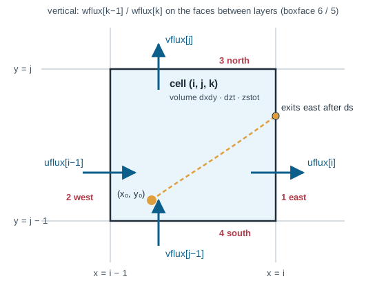
TRACMASS works on the staggered Arakawa C-grid. Tracers and cell volumes sit at the centre of each grid cell, and the velocity components sit at the centres of the cell faces: u on the east and west faces, v on the north and south faces, w on the faces between levels. TRACMASS does not use velocities directly. It uses volume fluxes through the faces (m³ s⁻¹), velocity times face area:

\[\begin{split} \begin{aligned} U_{i,j,k} &= u_{i,j,k}\,\Delta y_{i,j}\,\Delta z_{i,j,k}, \\ V_{i,j,k} &= v_{i,j,k}\,\Delta x_{i,j}\,\Delta z_{i,j,k}, \\ W_{i,j,k} &= w_{i,j,k}\,\Delta x_{i,j}\,\Delta y_{i,j}. \end{aligned} \end{split}\]

A GCM adapter computes these fluxes from the model’s velocities and grid metrics (see GCM adapters). Models on other Arakawa grids have to be moved onto the C-grid first. The Fortran documentation’s grid setup tutorial gives the A-to-C and B-to-C averaging formulas. The scrippsgog adapter shows how to move MITgcm’s west/south face staggering onto TRACMASS’s east/north faces.

Index conventions

Positions are continuous coordinates in units of grid cells:

• Cell ia (1-based, as in Fortran) covers ia - 1 <= x <= ia. Its west wall is at x = ia - 1 and its east wall at x = ia, and likewise for ja/y and ka/z.

• uflux[i, j, k] (0-based array index i = ia - 1) is the flux through the east face of cell ia, positive eastward. The west face of ia is uflux[i - 1]. With zonal periodicity (iperio = 1) the west face of the first column is the east face of the last.

• vflux[i, j, k] is the flux through the north face of cell ja, positive northward.

• Vertical flux. Adapters give wflux the way ocean models store it: wflux[i, j, k] is the flux through the top face of level k, positive upward (NEMO depthw, MITgcm WVEL). Inside LazyFluxFields and FluxFields it is converted to the kernel’s convention: the face between levels ka and ka + 1 (the bottom face of ka), positive towards increasing k, i.e. downward. That is w_kernel[..., k] = -wflux[..., k + 1], with zero below the deepest level. wflux is None in runs without vertical motion.

• kmt[i, j] is the number of ocean levels in each column. kmt == 0 marks land.

• Levels are numbered from the top: k = 1 is the first model level, and a level k > kmt is below the sea floor.

The “boxface” numbers in the figure are those of the Fortran code (mod_pos_tstep.F90): 1 east, 2 west, 3 north, 4 south, 5 and 6 for the two vertical faces.

Saved trajectories use the same coordinates. Cell i of a 0-based array covers i <= x < i + 1, with its centre at x = i + 0.5. gcm.glorys.xy_to_lonlat and tracmass.trajs.xy_to_lonlat convert these positions to longitude and latitude (see Coordinates).

The three-layer split

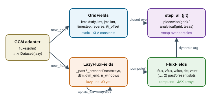
A trajectory run needs three kinds of data, which change at very different rates:

• the grid geometry (kmt, cell areas, sizes): fixed for the whole run;

• the velocity snapshots: change at every GCM output time and can be tens of gigabytes per snapshot for a global model;

• the particle state: changes at every sub-step.

TRACMASS-JAX keeps the first two in three objects, so the compiled kernel only has to be built once and flux data is only read when it is needed:

GridFields

Static geometry, built once per run by new_grid or new_flux:

Field	Shape / type	Description
kmt	(imt, jmt) int	Number of ocean levels; 0 on land
dxdy	(imt, jmt)	Horizontal cell area (m²)
imt, jmt, km	int	Grid size
timestep	pd.Timedelta	GCM output interval, always positive
reverse	bool	True for a backward run
iperio, jperio	int	Zonal periodicity, north fold (jperio = 1 is not supported yet)
i_offset, j_offset	int	Where the grid starts in the adapter’s full grid (subset i1, j1)

GridFields is a JAX pytree with kmt and dxdy as data. The kernel factories (advection_scheme.piecewise(grid), analytical(grid, tseas)) close over it, so kmt, dxdy and the sizes become constants in the compiled XLA program.

LazyFluxFields

The two-snapshot window of flux data, not yet read. It holds _past (slot 0) and _present (slot 1) dictionaries of xarray.DataArrays. For the reanalysis adapters these are Dask-backed, so no data has been read from disk. It also carries the run’s time stepping:

Field	Description
dtm	Time of the past (slot 0) snapshot
timestep, reverse	Copied from the grid
dtm_end	End of the run, as given to new_flux
n_windows	Windows left until dtm_end: ceil(abs(dtm_end - dtm) / timestep), or None
fluxes_fn	The adapter function, used by update_flux to open the next snapshot

Two operations act on it:

• lazy.compute() reads both slots and returns a FluxFields. It keeps the present slot’s arrays, so after the next update_flux the new past slot does not have to be read again. Each snapshot is read from disk once.

• update_flux(lazy) moves the window one timestep: present becomes past (a dictionary reference swap, no I/O), and the adapter is called for the next snapshot, which again only opens it lazily. This is the counterpart of Fortran’s swap_time in mod_swap.F90.

For backward runs update_flux steps backward in time, and uflux, vflux and wflux are negated lazily, so particles move upstream. Both new_flux and update_flux also convert wflux to the kernel convention (see Index conventions). The adapters always return forward fluxes.

FluxFields

The computed window, a JAX pytree passed to the kernel as a dynamic argument:

Field	Shape	Description
uflux	(imt, jmt, km, 2)	Zonal volume flux
vflux	(imt, jmt + 1, km, 2)	Meridional volume flux
wflux	(imt, jmt, km, 2) or None	Vertical volume flux, kernel convention (bottom face, positive down)
dzt	(imt, jmt, km, 2)	Layer thickness
zstot	(imt, jmt, 2)	Free-surface stretching factor (1 for fixed levels)

The trailing axis holds the two snapshots: index 0 is the past and index 1 the present. NaN and fill values in the fluxes are replaced by 0 when the data is read, which is the no-flow condition at land. The kernel accepts any FluxFields of the same shape and dtype without recompiling, so a new window costs only the read.

The key invariant

new_flux and update_flux never read flux data. Reading happens only in compute(), just before the kernel runs. After each window the integrator drops the computed arrays (del concrete; gc.collect()) so device memory is released before the next window is read. compute() warns if a window is larger than 8 GB, and suggests an [env.gcm] subset.

Building a grid

import tracmass
from tracmass import gcm

# Grid and buffer in one call (slot 0 is fetched once and shared)
grid, lazy = tracmass.new_flux(gcm.theoretical.fluxes, dtm_start="2007-06-01")

# A GCM can be given by name; [env.gcm] subset is applied first
grid, lazy = tracmass.new_flux("glorys", dtm_start="2010-06-01", dtm_end="2010-07-01")

# Build the grid once and reuse it for several buffers
grid = tracmass.new_grid("glorys", dtm_start="2010-06-01")
lazy_june = tracmass.new_flux(grid, "glorys", dtm_start="2010-06-01")
lazy_july = tracmass.new_flux(grid, "glorys", dtm_start="2010-07-01")

# Advance one window by hand
lazy = tracmass.update_flux(lazy)

With dtm_end earlier than dtm_start the run is backward: grid.reverse is True and the fluxes are negated. When you reuse a grid, new_flux checks that the dtm_end you pass agrees with grid.reverse.